import pysal as ps
import numpy as np
import pandas as pd
import matplotlib.pyplot as plt
import geopandas as gpd
%matplotlib inline

This is just a quick demonstration of what I understand from Hodges & Reich (2010)’s argument about the structure of spatial error terms. Essentially, his claim is that the substantive estimates ($\hat{\beta}$) from an ordinary least squares regression over $N$ observations and $P$ covariates:

$$ Y \sim \mathcal{N}(X\hat{\beta}, \sigma^2)$$

might not be equal to the estimates from a specific type of spatial autoregressive error model, such as the SAR error model:

$$ Y \sim\mathcal{N}\left(X\hat{\beta}, \left[(I - \lambda \mathbf{W})’(I - \lambda \mathbf{W})\right]^{-1}\sigma^2\right) $$

when (and only when) the filtered error term $(I - \lambda \mathbf{W})^{-1}\epsilon$ (for gaussian $\epsilon$ with dispersion $\sigma$) is correlated with at least one $X_j$, $j = 1, 2, \dots, P$.

Hodges & Reich (2010) consider a CAR model, but they argue (and I agree): the logic of the issue applies generally. The idea also touches on LeSage & Fischer (2008)’s argument motivating a spatial Durbin regression as “accounting for spatially-patterned ommitted covariates,” (Section 2.1, effective around page 280).

It’s pretty simple to show how it might affect regression below, so I’ve cooked up a short example using the Baltimore data. I think it’s important to understand this (just like apparent variance inflation in simulation designs due to $tr(\left[I - \lambda \mathbf{W}\right]^{-1}) \geq N$).

This is just one of those areas where, in theory, a “well-behaved” statement leads to results we’d want (identical estimates of $\beta$ between OLS and spatial error models), but when we use these models in reality, we must accept that empirical conditions will degrade these expectations.

So I’ll illustrate it on a standard PySAL dataset below, trying to show it as simply as possible.

Spatial Confounding in Spatial Error Models

Let’s consider the Baltimore house price dataset:

data = gpd.read_file(ps.examples.get_path('baltim.shp'))

Grab a symmetric spatial kernel weight, using a triangular kernel (but you can change it to be whatever you’d like), and ensure that the diagonal is zero, since that’s necessary for the spatial weights used in the spatial regressions in PySAL.

weights = ps.weights.Kernel.from_dataframe(data, k=10, fixed=True, function='triangular')
weights = ps.weights.util.fill_diagonal(weights, 0)

data.head()

.dataframe tbody tr th {
    vertical-align: top;
}

.dataframe thead th {
    text-align: right;
}

I’ll pick a subset of covariates that tries to avoid clumping/restriction of values, but give a decent enough model fit.

covariates = ['NROOM', 'AGE', 'LOTSZ', 'SQFT']

X = data[covariates].values
Y = np.log(data[['PRICE']].values)
N,P = X.shape

Now, I’m going to fit the ML Error model and the OLS on the same data.

mlerr = ps.spreg.ML_Error(Y,X, w=weights)
ols = ps.spreg.OLS(Y,X)

/home/ljw/anaconda3/envs/ana/lib/python3.6/site-packages/scipy/optimize/_minimize.py:643: RuntimeWarning: Method 'bounded' does not support relative tolerance in x; defaulting to absolute tolerance.
  "defaulting to absolute tolerance.", RuntimeWarning)
/home/ljw/anaconda3/envs/ana/lib/python3.6/site-packages/pysal/spreg/ml_error.py:483: RuntimeWarning: invalid value encountered in log
  jacob = np.log(np.linalg.det(a))

And, I’ll take a look at the two sets of estimates between the two, as well as computing the difference.

diff = (ols.betas - mlerr.betas[:-1]) 
distinct = np.abs(diff.flatten()) > (2*ols.std_err)
compare = pd.DataFrame.from_dict({"OLS" : ols.betas.flatten(), 
                        "ML Error" :   mlerr.betas[:-1].flatten(),
                        "Difference" :   diff.flatten(),
                        "SE OLS": ols.std_err,
                        "SE ML Error": mlerr.std_err[:-1],        
                        "Is Point-Distinct?" : distinct.astype(bool).flatten()})
compare.index = (['Intercept'] + covariates)
compare[['OLS', 'ML Error', 'Difference', 'SE OLS', 'SE ML Error', 'Is Point-Distinct?']]

.dataframe tbody tr th {
    vertical-align: top;
}

.dataframe thead th {
    text-align: right;
}

While the estimates are not interval-distinct (in that all interval estimates overlap), the point estimate from the ML Error regression for the lot size & age covariates do indeed fall outside of the interval estimate of the OLS.

Regardless, the $\beta$ are definitely “changed,” since their differences are well above the order of numerical precision. While this data is too noisy to show a really dramatic difference, it’s dramatic enough for two point estimates to fall outside the 95% confidence interval of another.

What’s Collinearity got to do with it?

OK, so I can show that they’re probably changed. And, if Hodges & Reich (2010) are right about this being a collinearity problem, I can show how changed they are by trying to orthogonalize my regressors.

1. So, I’m going to draw an $N \times N$ random matrix whose vectors are orthogonal.
2. Then, I’m going to construct a fake Y given the same $\beta$ from the OLS above.
3. If it’s true that the ML Error and OLS return the exact same betas when the error term is not collinear with the covariates, then in this construction, the OLS on the synthetic orthogonal data should recover the same betas as the OLS on the real data. Further, the OLS on the synthetic orthogonal data should also recover the same betas as the ML Error on the synthetic orthogonal data.

import scipy.stats as st

We can use scipy.stats.ortho_group to draw $N \times N$ matrices of orthogonal vectors. Taking the first $P$ of these will result in a synthetic $X$ matrix with orthogonal covariates. I’ll also add some uniform noise between -1,1.

Xortho = st.ortho_group.rvs(weights.n)[:,1:P+1] + np.random.uniform(-1,1,size=(N,P))

Then, I’ll use the same betas from the previous “real” problem to construct a $Y$:

inherited_betas = ols.betas

Yortho = Xortho.dot(inherited_betas[1:]) + inherited_betas[0] + np.random.normal(0,ols.sig2**.5)

Now, we run the regression and get the $\hat{\beta}$ coefficients:

ols_ortho = ps.spreg.OLS(Yortho, Xortho)
betas_from_ols_orthogonal_data = ols_ortho.betas

And we run the error model, too:

mlortho = ps.spreg.ML_Error(Yortho, Xortho, w=weights, method='ord')
betas_from_error_orthogonal_data = mlortho.betas

Now, are they all equal to within machine precision?

pd.DataFrame(np.column_stack((betas_from_ols_orthogonal_data,
                 betas_from_error_orthogonal_data[:-1],
                 inherited_betas)), columns=['Orthogonal OLS', 
                                             'Orthogonal ML Err', 'Observed OLS'])

.dataframe tbody tr th {
    vertical-align: top;
}

.dataframe thead th {
    text-align: right;
}

pd.DataFrame(np.column_stack((betas_from_ols_orthogonal_data,
                 betas_from_error_orthogonal_data[:-1], 
                 inherited_betas)), columns=['NA', 'Ortho. OLS minus Ortho. ML Error', 
                                             'Ortho. ML Error minus Observed OLS']).diff(axis=1).dropna(axis=1)

.dataframe tbody tr th {
    vertical-align: top;
}

.dataframe thead th {
    text-align: right;
}

Yep, those errors for the substantive effects are down in the $10^{-13}$ range, meaning the estimates are effectively within machine error in Python. The intercept between the orthogonal estimates and the non-orthogonal one looks slightly different, but this might be due to numerical issues in the estimation routines, since we’re using perfectly orthogonal covariates.

At the end of the day, what’s collinearity got to do with it? Below, I’ll plot the regressors in $X$ against the error term in the spatial error model:

import seaborn.apionly as sns
sns.pairplot(x_vars=covariates, y_vars='error_model_residual', 
             data=data[covariates].assign(error_model_residual = mlerr.u),
             kind='reg', plot_kws=dict(color='k', marker='.', line_kws=dict(color='orangered', zorder=100)))

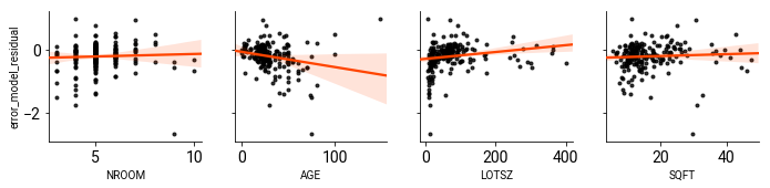
If you recall, the two covariates that had the largest shift from the OLS model to the ML Error model in the empirical dataset were the ones for house age and lot size. These are also marginally correlated with the residual from spatial error model.

However, in the case of the forced-to-be-orthogonal variates, they’re forced to be uncorrelated with the residuals.

Conclusion

Hodges & Reich (2010) demonstrate that, as this collinearity gets worse between elements of $X$ and the residual term in a spatial error model, the beta effects will change more and more dramatically.

Further, as I hope this shows, Hodges & Reich (2010), Section 2.5, is true for SAR models. There, they argue that

… spatial confounding is not an artifact of the ICAR model, but arises from other, perhaps all, specifications of the intution that measures taken at locations near to each other are more similar than measures taken at distant locations. (p. 330).

The crux of the issue is the collinearity between the correlated error and the $X$ matrix. If $X$ is collinear with the anticipated structure of $(I - \lambda W)^{-1}$, then $\hat{\beta}$ must change.

This is demonstrably true in the SAR Error example above. When using “raw” data with spatial multicollinearity, the use of an Error model changes the $\beta$ effects. While it doesn’t change them dramatically enough to overcome the standard errors, point estimates are disjoint. When using orthogonal covariates, the estimated effects are exactly the same (within machine precision) between OLS and SAR-Error models.