If you’ve ever tried to draw a tight boundary around a cloud of geographic points, you’ve probably met the convex hull — the rubber-band-stretched-around-all-the-points shape that’s fast and clean, but rarely tells the full story. Real-world data is lumpy, stretched, and full of gaps. What you usually want is a concave hull: a shape that hugs your data more closely, dipping inward where the points pull away. Fortunately, geopandas gives us ways to calculate both easily: the GeoSeries.concave_hull() method and GeoSeries.convex_hull attribute both can be used to recover these shapes quickly.
The trouble is, there’s no single “correct” concave hull. Too aggressive, and you get a spiky, fragmented mess. Too conservative, and you’ve just recalculated the convex hull.
Normally, the ratio parameter in GeoDataFrame.concave_hull() is used to solve this, but I find that getting that parameter right the first time is very unintuitive.
When I worked with @darribas a while ago to implement similar functionality in libpysal, I found directly modifying the alpha parameter to be more intuitive, since that represented “real” distances between points.
But, I want to use the new .concave_hull() functionality, since we’re probably going to deprecate that old alpha_shape()/alpha_shape_auto() code.
So, I was trying to solve this problem myself, and ended up with this approach. I didn’t see it documented anywhere, so I thought a short technical blogpost would be helpful.
My algorithm below finds a sweet spot — a smooth, well-enclosed boundary — by optimising a simple but useful geometric score.
What makes a concave hull “pretty”?
To find a good concave hull, we need to be able to score one. I think a “pretty” concave hull reflects a balance between how much empty area it omits from the convex hull and how irregular the boundary needs to be in order to omit this area. So, I thought back to my dissertation work and came up the following scores:
1. The Enclosure Ratio
The enclosure ratio is an areal measure of how effectively the concave hull “squeezes” area out of the concave hull for an equivalent set of points.
$$\text{enclosure ratio} = 1 - \frac{\text{candidate hull area}}{\text{convex hull area}}$$
This measures how much area the candidate hull encloses relative to the convex hull. A score near 0 means the concave hull covers almost as much area as the convex hull — it’s barely doing any concave-hugging. A score near 1 means the hull has shrunk dramatically, cutting out large swathes of empty space.
2. The Boundary Amplitude
The boundary amplitude is a previously-published score that measures how wiggly the perimeter of the concave hull is:
$$\text{boundary amplitude} = \frac{\text{convex hull perimeter}}{\text{candidate hull perimeter}}$$
This measures how indented or wiggly the candidate hull’s boundary is. The convex hull has a minimal, smooth perimeter, so this ratio starts at 1 and decreases as the concave hull develops more intricate, folded edges. A lower score means the boundary is increasingly jagged.
Perimeter Efficiency as a “prettiness” metric
These two metrics pull in opposite directions. Carving out more area (good enclosure ratio) tends to create more indented, complex boundaries (poor boundary amplitude). Using the weighted harmonic mean between these two scores lets us specify how much we care about covering the convex hull’s full area:
$$PE = \left(\frac{1-w_\text{area}}{\text{enclosure ratio}} + \frac{w_{\text{area}}}{\text{boundary amplitude}}\right)^{-1}$$
The harmonic mean is a natural choice here for a few reasons:
- It’s bounded between 0 and 1, giving a clean, interpretable score.
- It’s convex, meaning it has a well-behaved optimum to search for.
- Crucially, it penalises extremes hard. If either metric collapses — say, the boundary becomes a tangled mess — the overall score tanks. This pushes the optimiser toward solutions that are reasonably good on both fronts, rather than perfect on one and terrible on the other.
Given a weight $w_{\text{area}}$, optimising the perimeter efficiency score $PE$ lets us draw a “pretty” concave hull first try, without manually inspecting many concave hulls.
I find that an area weight of about .8 (so, we care about coverage 4 times more than convexity) helps set a reasonable prioritization.
Code for Pretty Concave Hulls
import geopandas
from scipy.optimize import minimize_scalar
from shapely.constructive import convex_hull

def pretty_concave_hull(
    multipoint,
    area_weight=.8,
    return_optimize=False,
    **optim_params
):
    if isinstance(multipoint, (geopandas.GeoSeries, geopandas.GeoDataFrame)):
        return pretty_concave_hull(
            multipoint.geometry.union_all(),
            area_weight=area_weight,
            return_optimize=return_optimize,
            **optim_params
        )
    if multipoint.geom_type != "MultiPoint":
        raise ValueError(f"geom type must be MultiPoint. Recieved {geoms.geom_type}")
    geoms = geopandas.GeoSeries(multipoint)
    vexhull = convex_hull(multipoint)
    def score(ri):
        cavehull = geoms.concave_hull(ratio=ri, allow_holes=False)
        ba = (vexhull.length/cavehull.length).item()
        fr = 1-(cavehull.area/vexhull.area).item()
        peff = ((1-area_weight)/fr + area_weight/ba)**-1
        return -peff
    opt_result = minimize_scalar(
        score,
        bounds=(0,1),
        **optim_params
    )
    if return_optimize:
        return opt_result
    else:
        return geoms.concave_hull(ratio=opt_result.x)
Example
from shapely.geometry import MultiPoint
import numpy as np
from matplotlib import pyplot as plt

# A crescent-shaped point cloud
angles = np.linspace(0, np.pi, 80)
noise = np.random.normal(0, 0.05, (80, 2))
coords = np.column_stack([np.cos(angles), np.sin(angles)]) + noise
coords = np.vstack([coords, coords + [0.3, 0]])

gdf = geopandas.GeoDataFrame(
    geometry=geopandas.points_from_xy(coords[:, 0], coords[:, 1]),
    crs="EPSG:4326"
)

pretty_hull = pretty_concave_hull(gdf)
default_hull = geopandas.GeoSeries(
  gdf.union_all()
).concave_hull()

# Plot
ax = gdf.plot(figsize=(8, 5), color="steelblue", markersize=10)
geopandas.GeoDataFrame(geometry=default_hull).boundary.plot(ax=ax, color="black", linewidth=2, label='default')
geopandas.GeoDataFrame(geometry=pretty_hull).boundary.plot(ax=ax, color="crimson", linewidth=2, label='pretty')
plt.show()
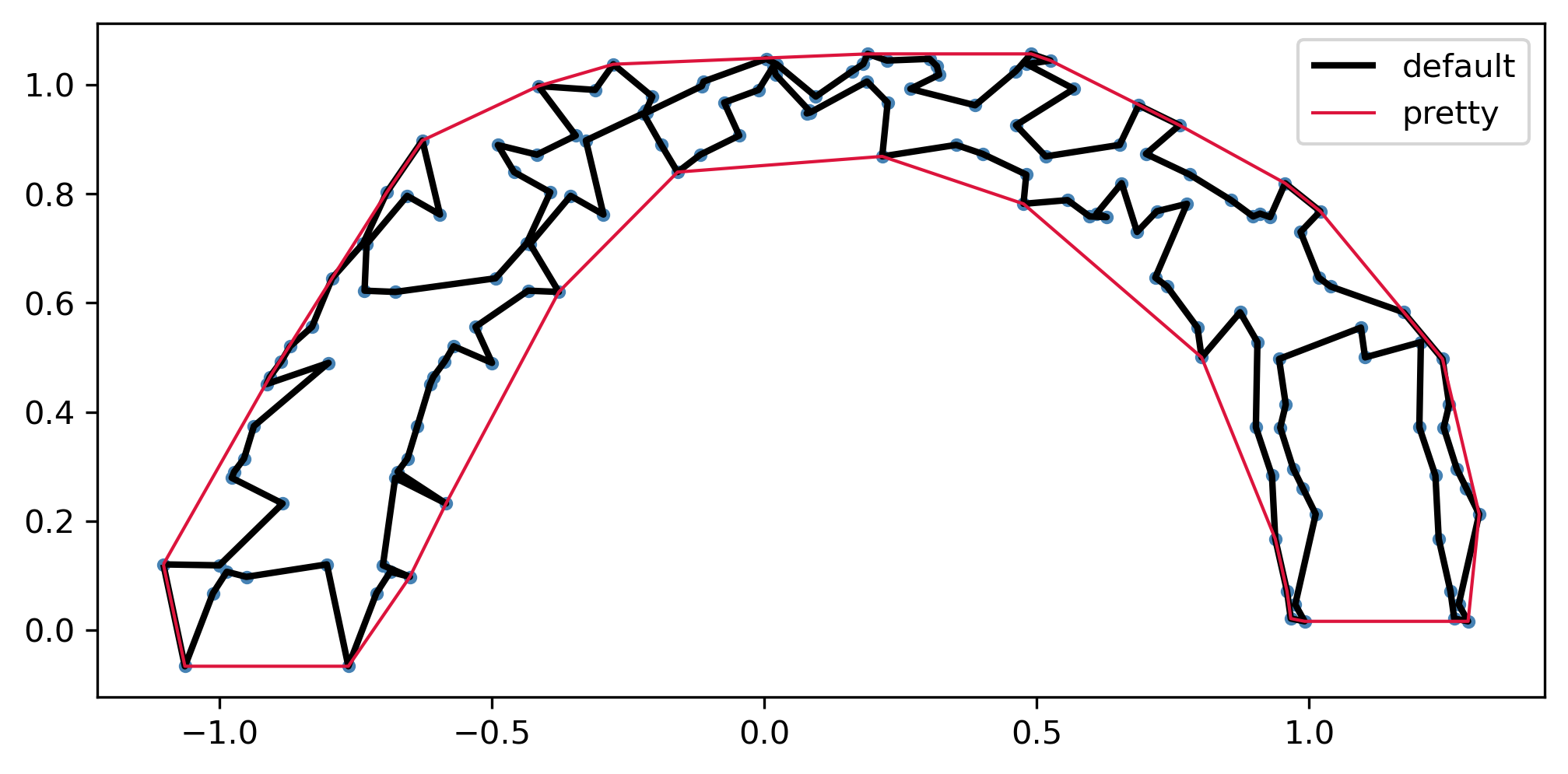
This heuristic with a 4:1 weight on the areal enclosure score (all in the code above) gives a hull that traces the crescent naturally — concave where the data dips away, without jagging into noisy spikes.